
Finding Incremental Lift With Geo-Experiments
When we run ads, we want to know that the ads are producing conversions that our business wouldn’t otherwise get. Since there is so much overlap between organic and paid listings in Google Ads, it isn’t always clear how many additional conversions we’re actually getting by running ads instead of just relying on free listings in Google. In other words, we don’t always know if the conversions we get from ads would get picked up by organic listings if we hadn’t run ads. One of the ways to measure incremental lift from advertising efforts is through geo experiments. With geo experiments, you divide up a set of geos (short for “geographic areas”) into control and treatment groups – for the treatment group you run ads and in the control group you keep everything constant. Then you compare conversion results between the two groups after you run ads for the treatment group. There are tools out there for designing these experiments and analyzing results: Facebook offers GeoLift, Google offers GeoexperimentsResearch, and Google offers Google Ads conversion lift studies. All of these offerings are very useful, although they can be difficult to get set up and running. Another, really easy option is to use Google Analytics with old-fashioned Excel spreadsheets.
Classical Linear Models Using ANOVA
ANOVA stands for analysis of variance. We’re taking repeated conversion measures – in a time period with ads and a time period without ads – of two groups (a categorical variable): geos that have ads running and geos without ads running. We combine the number of conversions for the two groups, basically looking at how the number of conversions changed over the two time periods. We analyze the amount of variance in the change in conversions we can explain by knowing if a geo had ads running or not. If the amount of variance we can explain is a lot compared to the amount of variance that remains unexplained, then we know that running ads makes a significant difference in conversion totals. Ultimately we’re answering the question “does running ads increase conversions significantly” by deciding if we can reject the null hypothesis: changes in conversions are not different for geos that run ads versus those that don’t. Mathematically this is what that looks like:
Model C: Ŵ1 = β0 = W̄
Model A: Ŵ1 = β0 + β1(TX)
The null hypothesis is H0 : β1 = 0.
Ŵ1 (“W” hat) is our calculated estimate for W1, the weighted average difference in conversions across time periods. W̄ (“W” bar) is the average of the weighted average of the combined conversion totals across all geos. Model C is the simplest model for predicting the value of the combined total for each geo – we’re estimating that the actual value for each geo is just the average across all geos. Model A is a bivariate regression (that Excel will calculate for us), which takes into account whether a geo was part of the group that had ads running or not. If adding that effect to Model C significantly improves our prediction for the value of the combined number of conversions (i.e. the conversion change from time period 1 to time period 2), then we can reject the null hypothesis, and β1≠ 0. This means that advertising made an incremental increase in conversions that would not have been picked up organically if ads had not been running.
Computing Error With Actual Data
Below are some actual data. TX indicates a geo’s treatment status: 1 = ran ads during T1 and -1 = did not run ads during T1. T1 is the sum of conversions for a 4 week period with ads running. T2 is the sum of conversions for a 4 week period without ads running. W1 is the weighted difference between T1 and T2: (T1 – T2)/√(2). That might look weird; why not (T1 – T2)/2 for finding an average difference? We’re using contrast codes. This is just a strategy that makes interpreting results easier because it tends to keep things centered around 0. We’re representing categorical variables numerically by assigning them either +1 or -1 and then normalizing them by dividing by the square root of their squares:
Here’s the data:
| Region | TX | T1 | T2 | T1 – T2 | W1 |
| Geo 1 | 1 | 11 | 13 | -2 | -1.4142 |
| Geo 2 | 1 | 11 | 9 | 2 | 1.4142 |
| Geo 3 | 1 | 101 | 68 | 33 | 23.3345 |
| Geo 4 | 1 | 110 | 75 | 35 | 24.7487 |
| Geo 5 | 1 | 44 | 42 | 2 | 1.4142 |
| Geo 6 | 1 | 56 | 56 | 0 | 0.0000 |
| Geo 7 | 1 | 50 | 40 | 10 | 7.0711 |
| Geo 8 | -1 | 5 | 11 | -6 | -4.2426 |
| Geo 9 | -1 | 18 | 13 | 5 | 3.5355 |
| Geo 10 | -1 | 113 | 109 | 4 | 2.8284 |
| Geo 11 | -1 | 95 | 102 | -7 | -4.9497 |
| Geo 12 | -1 | 34 | 44 | -10 | -7.0711 |
| Geo 13 | -1 | 66 | 48 | 18 | 12.7279 |
| Geo 14 | -1 | 55 | 62 | -7 | -4.9497 |
| Average | 54.9286 | 49.4286 | 5.5 | 3.8891 |
These are our actual values for W1. From here we want to look at how well our two models – Model C, the simple, compact model, and Model A, the model that takes into consideration advertising status – estimate W1. By analyzing the sum of squared error between the two models, we can see if Model A significantly reduces the amount of error that exists in Model C. Remember Model C is the simple model – it just uses the average of W1 across all geos (3.8891) to estimate the value of W1 for each individual geo. Here is the data, calculating the error for Model C:
| Region | W1 | Ŵ1 | (W1 – Ŵ1) | (W1 – Ŵ1)2 |
| Geo 1 | -1.4142 | 3.8891 | -5.3033 | 28.1250 |
| Geo 2 | 1.4142 | 3.8891 | -2.4749 | 6.1250 |
| Geo 3 | 23.3345 | 3.8891 | 19.4454 | 378.1250 |
| Geo 4 | 24.7487 | 3.8891 | 20.8597 | 435.1250 |
| Geo 5 | 1.4142 | 3.8891 | -2.4749 | 6.1250 |
| Geo 6 | 0.0000 | 3.8891 | -3.8891 | 15.1250 |
| Geo 7 | 7.0711 | 3.8891 | 3.1820 | 10.1250 |
| Geo 8 | -4.2426 | 3.8891 | -8.1317 | 66.1250 |
| Geo 9 | 3.5355 | 3.8891 | -0.3536 | 0.1250 |
| Geo 10 | 2.8284 | 3.8891 | -1.0607 | 1.1250 |
| Geo 11 | -4.9497 | 3.8891 | -8.8388 | 78.1250 |
| Geo 12 | -7.0711 | 3.8891 | -10.9602 | 120.1250 |
| Geo 13 | 12.7279 | 3.8891 | 8.8388 | 78.1250 |
| Geo 14 | -4.9497 | 3.8891 | -8.8388 | 78.1250 |
| SSC | 1300.7500 |
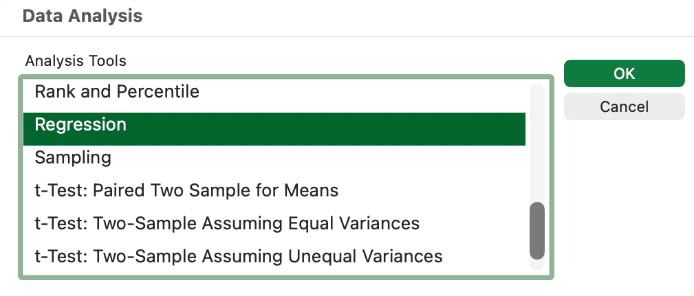
The error of Model C is 1300.75. To calculate the error for Model A, we need to complete the regression for Model A to get a value for β1. It’s not that hard to calculate it by hand for a bivariate regression, but either way, Excel has a built-in Data Analysis ToolPak that makes it even easier. This is how you install it. Calculate the regression by entering the data below in a spreadsheet, selecting Data Analysis > Regression, entering the W1 column for the “Y Range,” entering the TX column for the “X Range,” checking the box for “Labels,” and clicking “OK.”
| Region | W1 | TX |
| Geo 1 | -1.4142 | 1 |
| Geo 2 | 1.4142 | 1 |
| Geo 3 | 23.3345 | 1 |
| Geo 4 | 24.7487 | 1 |
| Geo 5 | 1.4142 | 1 |
| Geo 6 | 0.0000 | 1 |
| Geo 7 | 7.0711 | 1 |
| Geo 8 | -4.2426 | -1 |
| Geo 9 | 3.5355 | -1 |
| Geo 10 | 2.8284 | -1 |
| Geo 11 | -4.9497 | -1 |
| Geo 12 | -7.0711 | -1 |
| Geo 13 | 12.7279 | -1 |
| Geo 14 | -4.9497 | -1 |
This will create a new sheet in your workbook that has a bunch of data, including the data we are manually calculating here! You could just skip all the sum of squared error calculations we’re doing and grab the numbers from the ANOVA table it creates, but for the fun of it, we’ll also do it manually.
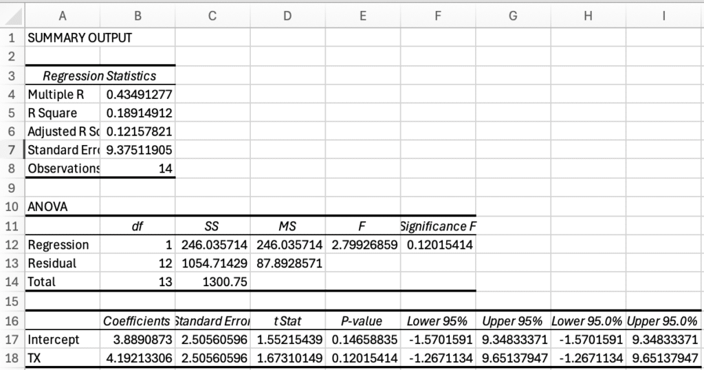
The part we’ll use are the coefficients for the intercept and TX. These are the values for our coefficients:
Model A: Ŵ1 = β0 + β1(TX) = 3.8891 + 4.1921(TX)
Notice that β0 is equal to the mean, W̄. This is from using contrast codes, and makes things a bit easier to interpret. Now that we have Model A, we can calculate the error for Model A and compare it to the error for Model C.
| Region | TX | W1 | Ŵ1 | (W1 – Ŵ1) | (W1 – Ŵ1)2 |
| Geo 1 | 1 | -1.4142 | 8.0812 | -9.4954 | 90.1633 |
| Geo 2 | 1 | 1.4142 | 8.0812 | -6.6670 | 44.4490 |
| Geo 3 | 1 | 23.3345 | 8.0812 | 15.2533 | 232.6633 |
| Geo 4 | 1 | 24.7487 | 8.0812 | 16.6675 | 277.8061 |
| Geo 5 | 1 | 1.4142 | 8.0812 | -6.6670 | 44.4490 |
| Geo 6 | 1 | 0.0000 | 8.0812 | -8.0812 | 65.3061 |
| Geo 7 | 1 | 7.0711 | 8.0812 | -1.0102 | 1.0204 |
| Geo 8 | -1 | -4.2426 | -0.3030 | -3.9396 | 15.5204 |
| Geo 9 | -1 | 3.5355 | -0.3030 | 3.8386 | 14.7347 |
| Geo 10 | -1 | 2.8284 | -0.3030 | 3.1315 | 9.8061 |
| Geo 11 | -1 | -4.9497 | -0.3030 | -4.6467 | 21.5918 |
| Geo 12 | -1 | -7.0711 | -0.3030 | -6.7680 | 45.8061 |
| Geo 13 | -1 | 12.7279 | -0.3030 | 13.0310 | 169.8061 |
| Geo 14 | -1 | -4.9497 | -0.3030 | -4.6467 | 21.5918 |
| SSA | 1054.7143 |
Analyzing the Variance From Our Example
Now that we have the amount of error from Model C and Model A, we can calculate how much introducing a parameter that accounts for whether a geo displayed ads or not can help explain the changes in the number of conversions across geos. We do this by calculating an F-ratio. The F-ratio calculates how much error we were able to reduce by introducing a new parameter compared to how much error is left on average for the remaining degrees of freedom. Degrees of freedom are the pieces of information being used in a model – it’s based on the sample size and the number of parameters in a model. If our goal is to reject the null hypothesis, we want a high F-ratio. It means that we were able to reduce the amount of variance a lot compared to the amount that is left in our model, so the parameters we introduced had a lot of explanatory power. By using Excel, we can look up the probability of getting a certain F-ratio if there’s no relationship between the change in conversions for a geo and whether a geo displayed ads. Basically it is referencing an F-distribution, which is a probability distribution that compares variances (mean square errors).
These are the sum of squared errors for our models:
| Model | Parameters | SSE |
| Model C | 1 | 1300.7500 |
| Model A | 2 | 1054.7143 |
| SSR | 246.0357 |
The “SSR,” or sum of squares reduced, is the difference in the sum of square errors between Model C and Model A. It is the amount that error was reduced by introducing a parameter for advertising status. Model A has two parameters: β0 and β1. Model C has just one: β0. This is important for determining the degrees of freedom (df) for our F calculation. The F-ratio is mean square error explained by Model A (MSB or Mean Square Between) divided by the mean square error that is left (MSW or Mean Square Within). Mean squares are calculated by dividing the sum of squared error by the degrees of freedom. For MSB, there is one degree of freedom because we added one parameter to reduce the amount of error by 246.0357. For MSW, there are 12 degrees of freedom because there were 14 geos and Model A used 2 parameters (14 – 2 = 12). Here are the calculations:
MSB = SSR/df = 246.0357/1 = 246.0357
MSW = SSA/df = 1054.7143/12 = 87.8929
F = MSB/MSW = 246.0357/87.8929 = 2.7993
Knowing the value for F, we can now look up the probability of having an F this large if the change in conversions from time one and time two does not depend on advertising status.
P = F.DIST.RT(2.7993,1,12) = 0.12
Typically in sciences, you only reject the null hypothesis if P ≤ 0.05. In this case, it is greater, so we accept the null hypothesis. The ads aren’t working; we’ll see these kinds of results 12% of the time if there is no relationship between running ads and the change in conversions. But maybe we can look at this a little closer. Rejecting the null hypothesis when it is true is called a Type I error. In the sciences, you really want to avoid making a Type I error. For example, let’s say you have some kind of medicine with side effects that may or may not help with some disease. You run an experiment and based on the data you reject a null hypothesis that taking the medicine has no effect on recovery rates (i.e. the medicine helps). Companies start manufacturing the medicine, and people start paying for it and taking it, but it turns out that you made a Type I error. You cost people money and expose them to negative side effects thinking you’re helping them recover from a disease, but it turns out the medicine doesn’t help. Pretty bad. In contrast, when you accept a null hypothesis when it is false, it is called a Type II error. If you decide your medicine doesn’t work, when it does help, that’s a Type II error. Also not good, but in this case, maybe more acceptable. Unlike in science, for marketing a Type I error is probably more acceptable than a Type II error. For example, your business is struggling and you’re trying to decide if ads are effective. You run an experiment and falsely conclude that ads don’t help. You stop advertising, mistakenly, and now your business is worse off because you made a Type II error. Probably, you would have rather made a Type I error in this scenario. When it’s more acceptable to make a Type II error than to make a Type I error, you might accept a larger threshold for P to reject H0.
F-test Vs T-Test Special Case
Originally we used an F-test to analyze the data, but we could also use a T-test. Whereas an F-test compares variances, a T-test compares two group means to determine if there is a statistically significant difference between the two. The advantage to using a T-test in this case is it has two-tail and one-tail variations. In this case we are only interested in a one-tail test. In a two-tail test we would reject the null hypothesis if the change in conversions was significantly higher or lower. But in this case, if the change in conversions was significantly smaller when we run ads compared to when we don’t, we’d accept the null hypothesis and say that advertising doesn’t affect the change in conversions. In other words, we are only interested in knowing if advertising increases conversions. For Google Ads, it’d be weird if running ads caused us to get fewer conversions overall (we’d have to be really bad at advertising), and we’re generally not interested in that possibility. Therefore we use a one-tail test.
When we’re only comparing one variable with two groups, the values for F and t are related: F = t2. We can use Excel to determine the probability that the weighted mean difference with ads vs without ads is significant:
P = T.DIST.RT(SQRT(F), df) = T.DIST.RT(SQRT(2.7993), 12) = 0.06
Now we have a P that is still larger than 0.05, but much closer to 0.05. It looks more reasonable to reject H0 (the null hypothesis), risking a Type I error. In other words, we’re unlikely to have a t value that is as large as it is, if ads didn’t increase conversions, so we conclude that advertising does impact our overall conversion total, resulting in incremental conversions.
Key Takeaways and Resources
Attribution can tell you where a conversion came from, but incrementality tells you whether it would have happened at all. If you want help turning experiments like these into a reliable strategy, from designing geo tests to improving ROI and measuring lift , explore our PPC management services or dig into tools like the PPC ROI calculator to quantify effectiveness in your own campaigns. And if you’re looking to strengthen your organic foundation so that paid and free traffic work together more efficiently, check out our SEO services. For more education like this post, head over to the Pure Visibility blog for actionable insights you can use today.